Quantitative analysis of fatigue fracture
The microscopic feature analysis of fatigue fractures for failure analysis always hopes to find the relationship between microscopic features and macroscopic cracking factors and macroscopic fracture behavior. And to quantitatively determine the impact of various factors on the fracture accident. In order to improve the accuracy of accident diagnosis.
The relationship between microscopic fatigue striation and crack growth rate has been deeply studied, and many practical results have been achieved so far. Microscopic analysis of fatigue fractures is used to quantitatively obtain crack growth rate, fatigue life, and even estimate fatigue load and cyclic fatigue fracture toughness of materials. The task of quantitative analysis of fatigue fractures is to quantitatively estimate the above parameters from the fatigue-trim characteristics, study the factors affecting the reliability of quantitative analysis, and analyze the existence and effective conditions of quantitative analysis.
First, the crack growth rate and fatigue life are estimated by the fatigue striation spacing.
We know that the width and number of fatigued ridges are a function of the cyclic load level and the number of cycles. On the other hand, the fracture mechanics analysis believes that the fatigue crack growth rate (da/dN) of the macro ship is a function of the crack stress intensity factor range (ΔK). In many cases, the number of striations on the fatigue fracture is one-to-one corresponding to the number of load cycles, and the width of the fatigue striation is increased as the stress level increases. At the same time, as the length of the crack increases, the width also increases accordingly. See Figure 6-68. In this case, the micro-crack propagation rate (da/dN) calculated from the width of the crease on different parts of the fracture (ie different crack depths) can be regarded as a comparison with the mechanical test of the macro ship. The macroscopic crack growth rate (da/dN)) macro is consistent. This allows the fatigue life of the part to be estimated by means of the width of the crease on the fracture.
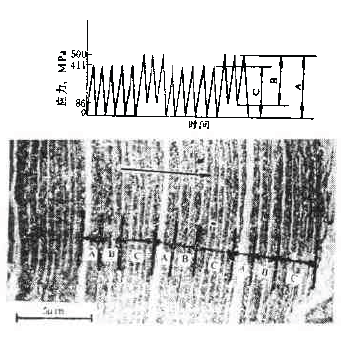
Figure 6-68 Correspondence between fatigue fringes and cyclic stress of 2017-T4 aluminum alloy and the effect of cyclic stress level on the striation pitch (arrow shows the direction of crack propagation)
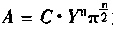
The empirical formula of the fatigue crack growth rate proposed by paris shows that the crack growth rate is controlled by the stress intensity factor range ΔK of the crack tip, namely:
Where C, n are the constants of the material, respectively
Where r is a shape factor.
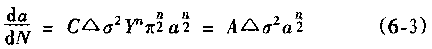
From (6-1) and (6-2)
In the middle
 Is a constant term.
 Equation (6-3) shows that when the applied stress is constant, the fatigue crack growth rate is a crack.
An exponential function of length a, ie

In the special case of n=2
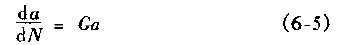
That is, there is a linear relationship between da/dN and a.
Equation (6-4) shows that we can bypass the mechanical parameters (â–³K) and material constants that are difficult to obtain in practical problems, obtain the relationship of da/dN -a directly from the fatigue fracture, and estimate the fatigue life. Specific steps are as follows:
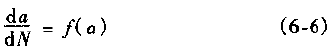
1. The fatigue striation width is measured from the fracture source region to different portions of the expansion direction on a1, a2, a3, ... (i.e., different crack lengths). In order to reduce the measurement error, the total width of several to several tens of striations can be measured, and then the average value is taken, which is the crack growth rate da/dN of the portion. The method is shown in Figure 6-69.
2. According to the da/dN value corresponding to each length a, the da/dN-a curve can be obtained by a suitable fitting method, as shown in Fig. 6-70. According to the shape of the curve, the appropriate analytical method can be used to find the analytical relationship between da/dN and a, ie
In many cases, the formula (6-6) is an exponential function, and in some cases, a linear relationship may be present.
3. Calculate the fatigue life of the fatigue crack from the initial length ai to the fracture length ac according to the formula (6-6), ie
Figure 6-69 shows a schematic diagram of the determination of da/dN on fractures with different crack lengths. Figure 6-70 shows the da/dN-a curve based on the measured data.
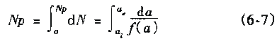
The Np value can be obtained by substituting the specific mathematical expression of f(a) into the equation (6-7) by the analysis of the da/dN-a curve. Here, Np is the fatigue life of the fatigue crack growth period, and the sum of the fatigue crack initiation life Ni is the total life of the fatigue fracture of the part. For parts with good surface quality and no crack or crack-like defects, other methods should be used. Ni is obtained, and for a large number of actual parts that are caused by "innate" surface cracks or crack-like geometry and surface-caused fatigue crack propagation and failure, the crack-like end is used (6-7) The Np value is the total fatigue life Nf of the part.
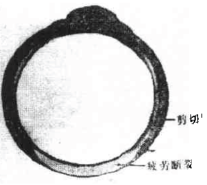
Figure 6-71 Macro fatigue fracture morphology of aluminum alloy cylinder
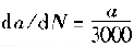
Figure 6-71 shows the fatigue fracture of an aluminum alloy cylinder. The fatigue source is initiated on the inner wall of the cylinder and then spreads to the outer surface and both sides. The fatigue expansion zone is a flat fracture, and the instantaneous fracture is a shear oblique fracture. Figure 6-72 shows the SEM image of the fracture at distances of 1. 0, 1.5, 3.0 and 5.0 mm from the inner wall surface of the cylinder. The rate of crack propagation over each crack length can be calculated from the fatigue-wrist spacing on the graph, as shown in 6-73. According to the linear relationship of the graph
 or
or 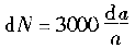
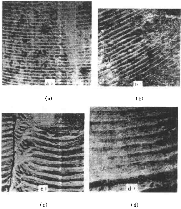
Figure 6-72 SEM image of a different depth of the fracture from the inner wall surface
(a) 1.0 mm; (b) 1.5 mm; (c) 3.0 mm; (d) 5.0 mm 2745 ×
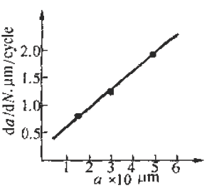
Figure 6-73 da/dN-a relationship curve calculated from the striation spacing on Figure 6-72
The life of the crack from 1 mm to mm (wall thickness) was calculated from the above formula to be 4,828 cycles. This is very close to the number of cycles of 4,904 cycles that occur when the cylinder is in use.
Quantitative analysis of fatigue crack growth rate and fatigue life by this method is intuitive and simple, and is very meaningful for failure analysis in engineering. However, it should be noted that the calculation method is based on the ideal expansion mode, and the actual fatigue fracture situation has complex problems. If the treatment is not good, the quantitative analysis results will be seriously distorted, and in some cases, it will be helpless. It is necessary to study the characteristics of various types of fatigue fractures in depth, summarize the effects of various solid factors, and find ways to correct various possible errors, and try to reduce the gap between the calculation results and the real situation. At present, people find that they should pay attention to There are several problems.
(1) The formula (6-7) establishes the relationship between the crack propagation length and the number of cycles in the second stage of crack propagation, and the fatigue fracture problem mainly based on the second stage expansion has sufficient reliability. However, for the first stage (including the crack initiation period), which account for a large proportion of the fatigue life, the number of cycles (life) calculated by this method will have a considerable gap with the actual life, and it is difficult to borrow This extrapolated total life.
(2) When applying the formula (6-7), the key is to determine the formula (6-6). It is easier to determine this relationship in the second expansion stage of some materials, and the crack spreads to the near-instantaneous region, that is, the expansion. When it is sufficient to produce a toughness-fatigue fracture, many dimples will gradually appear in the fracture. In this case, first, the fatigue glow is difficult to accurately measure, and second, some of the phases of some materials have no exact correspondence between the fatigue fringe spacing and the number of loading cycles in the region. For example, the β phase (body center cube) in the fatigue fracture of carbon steel and manganese bronze does not maintain a good one-to-one correspondence like the α phase (face centered cubic) in bronze. This makes quantitative analysis extremely difficult. As for the materials that do not have fatigue fringes at all, it is impossible to establish the relationship between the fatigue fringes and the number of cycles.
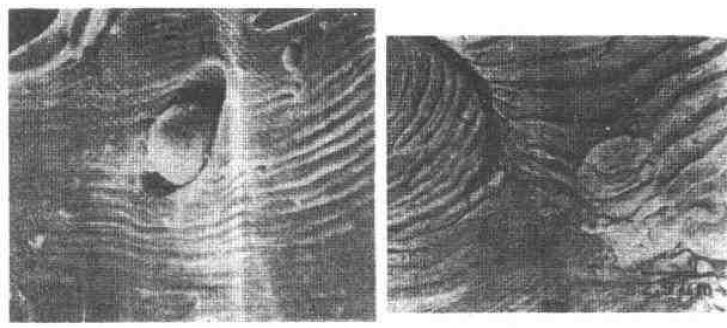
(3) When there are inclusions in the material, the fatigue ridges will not be able to maintain a uniform parallel feature. The ridges will wrap around or continue inside the inclusions, so that the expansion rate of the local area is greater than the average rate. See Figure 6-74
(a) (b)
Figure 6-74 (a) Fatigue and striated roundabout around the genus or continue to the top
(b) Example of the fatigue wrinkle spacing of the same part on the fracture of the 718 alloy notched specimen
(4) The contour analysis of the fatigue fracture of 45 steel proves that the fatigue fringes of each micro-area are not strictly perpendicular to the maximum tensile stress, and most of the sections are oriented in the range of 45-90° to 65°. For the most. The main crack is perpendicular to the main tensile stress. Thus, when using the local embossing juice to calculate the main crack growth rate, the directional factor must be considered to complicate the method.
(5) Due to different crystallographic orientations, the fatigue fringes of different micro-segments are not only oriented differently, but also the fatigue fringe spacing is also significantly different, some differences can be up to five times, Figure 6-74(b) is an obvious An example.
(6) Generally speaking, the fatigue striation pitch will increase uniformly with the increase of crack length, but few materials can maintain a linear relationship. Experiments on Cr18Ni10Ti steel and No. 20 steel, 35CrNi3MoA. In the two stages of crack propagation and the like, the width of the microscopic fatigue striation does not change much, ranging from about 0.5 μm (starting end) to 1.25-1.5 μm (terminal). However, in the mixed fracture zone adjacent to the short-cut zone, the micro-fatigue striation width will increase sharply. For example, for Cr18Ni10Ti steel, the pitch of the second stage extension zone is about 1.5 μm, and if the crack grows by 1.5 mm. The pitch of the crepe will increase by nearly ten times, that is, about 14 μm, which may be caused by the transition of the stress state when the crack propagates to the critical dimension of instability. Figure 6-75 illustrates the relationship between crack length and microscopic fatigue striation width. In the actual quantitative analysis, the segmentation of the observation segment is encrypted for the segment where the variation of the ridge width is intense.
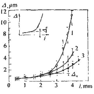
Figure 6-75 Relationship between fatigue striation spacing and crack length in steel 1-Cr18Ni10Ti; 2-35GrNi3MoA; 3-20 steel
(7) Experience has shown that the reliability of quantitative analysis is also related to the magnitude of crack growth rate. For general tough materials, regardless of the type of material, if the expansion rate is in the range of 0.1 to 1 μm/time, the macroscopic crack growth rate by the formula (6-6) has sufficient reliability.
When the crack growth rate is >1μm/time, the fatigue crepe spacing is generally smaller than the crack growth rate, which occurs mostly in the section of the section that transitions from the steady-state crack propagation (second stage) to the instability expansion. There are already dimple patterns on it. The rate of expansion calculated from the fatigue striation spacing reflects only a portion of the expansion and does not reflect the effects of the dimple.
When the crack growth rate is <0.1 μm/time, contrary to the above, the fatigue crepe pitch is larger than the crack growth rate. This is mainly the result of grain orientation and material structure. When the crack meets the grain boundary and the phase interface of the second phase. The crack will temporarily stop expanding and the expansion rate will be reduced. In this area, the section often has irregular embossing patterns, or intergranular fractures caused by materials and environmental atmospheres, and brittle sections of river patterns.
(8) The reliability of quantitative analysis is also related to the fracture toughness of the material. Generally speaking, as the fracture toughness of the material decreases, the difference between the crack growth rate and the fatigue striation spacing will increase. As long as the fracture toughness value K1c is high, even a material with a high tensile strength can ensure good reliability, and fracture toughness is a material property that has an important influence on quantitative analysis.
For high-hard materials, such as bearing steel, ultra-high-strength steel, etc., fatigue wrinkles are not observed, so this method cannot be used for quantitative analysis.
(9) Fatigue fractures often appear similar to fatigue fringes, but in fact they are not fatigued pattern or true fatigue and non-fatigue pattern, as shown in Figure 6-76. The more regular average line is not fatigue fringes, it may be a series of parallel straight cracks composed of severe local embrittlement of the matrix.
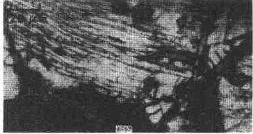
Figure 6-76 Cast aluminum alloy fracture, micrograph
The pattern on the upper left of Figure 6-77 is definitely not a fatigue glow pattern. It may be a pattern related to the crystal structure. Figure 6-78 shows a clear fatigue pattern, but the pattern on the right side of the dark area is the cleavage step. Rather than fatigue. In Figure 6-79, the center portion shows irregular fatigue lines (A and B), and the fine pattern on the facet at C is not an illusion or glow, which may be caused by the matching fracture surface wear. The fatigue pattern in Figure 6-80 is extremely irregular and is accompanied by a dimple morphology. Figure 6-81 shows a small face that is much like the plane along the cleavage plane, but the parallel pattern may not be the fatigue glow, but the morphology of the foot associated with the oxide film.
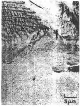
Figure 6-77 Photograph of the fatigue fracture of Waspaloy alloy
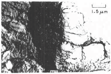
Figure 6-78 Micrograph of fatigue fracture of 302 stainless steel sheet
Figure 6-79 Photograph of fatigue fracture of V-700 alloy Figure 6-80 Micrograph of fatigue fracture of 431 stainless steel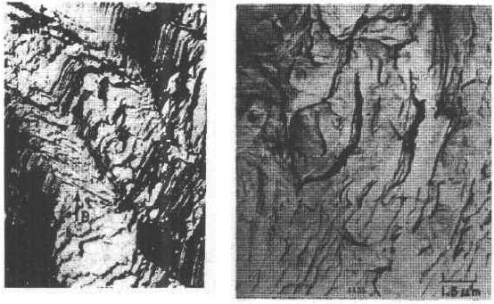
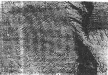
Figure 6-81 Microscopic picture of fatigue fracture of 302 stainless steel
Figure 6-82 shows the fracture morphology of the 4340 steel after loading and breaking. It is not a fatigue fracture, but the surface shows fine chopping texture, which may be due to the fracture of the fine pearlite layer. In this case, it is necessary to pay attention to discrimination, otherwise it is easy to misjudge the fatigue fracture. In addition to the problems in the original analysis of the above fractures, it should be noted that the quantitative determination of fatigue life by fracture analysis technology is a reverse analysis method. Due to the uncertainty of many factors and the randomness of crack propagation, the quantitative analysis results can only be In the prediction interval under certain confidence, there are many statistical problems that need to be carefully dealt with throughout the analysis.
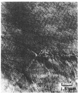
Figure 6-82 Micrograph of 4340 steel static load breaking fracture
From the above introduction, it can be seen that the quantitative analysis of actual fatigue fractures is quite complicated and difficult. This requires that fracture analysts not only have to study the theoretical results of fatigue micro-fracture analysis, but also pay attention to the analysis of actual fractures through a large number of fractures. With accumulated experience, we can handle all kinds of complicated problems handily. In the specific study of a fatigue fracture problem, it is necessary to take a few microscopic pictures along the direction of crack propagation, pay attention to the problems that need to be paid attention to in the above points, and do a comprehensive analysis work to avoid the partial cover and the falsehood.
Second, the fatigue intensity is used to measure the stress intensity factor amplitude and fatigue load
The research results of fracture mechanics have proved that the stress intensity factor K is a main parameter controlling the crack growth rate. A lot of research work has been done on the relationship between the crack growth rate da/dN and the stress intensity due to the amplitude ΔK, and a certain relationship has been established. In general, the double logarithmic coordinates of the relationship between da/dN and ΔK It can be divided into three areas. Zone II is the effective interval of the paris formula. As shown in Figure 6-83, there is an eigenvalue at both ends of the interval. The △Kth of the front end is called the threshold value, which is the minimum stress intensity factor that satisfies the application condition of the paris formula. When the neighboring edge ΔKth, the small decrease da/dN of ΔK sharply decreases. The characteristic value Kc of the end is the maximum stress intensity factor satisfying the application condition of the paris formula, and is an upper limit value when Kmax→K1c, that is, a critical value of the transition from subcritical to unstable expansion.
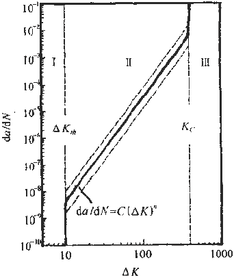
Figure 6-83 â–³ K-da / dN relationship
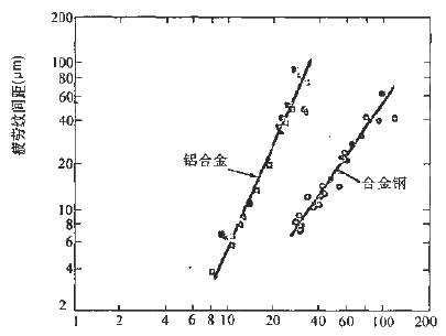
On the other hand, the results of fatigue fracture analysis have proved that the relationship between conventional mechanical properties and stress levels and fatigue striations is very poor. For example, some materials vary greatly in strength and have the same spacing under the same △K. Fatigue shine. It can be seen that the relationship between the fatigue striation pitch and the conventional mechanical properties is very uncertain, and it has a good correlation with △K. For series alloys with different strength indexes, they have the same fatigue striation spacing when the stress field strength factor ΔK is constant. This relationship can be expressed in the same form as the paris formula in fracture mechanics μ=A[△K]n (6-8) where μ is the fatigue striation width, A and n are stress-dependent material constants, and stress states Irrelevant, regardless of the sample size, the n value is 2.5 for aluminum and 1.6 for steel.
Figure 6-84 shows the double logarithmic coordinate curve and test point of the relationship between the fatigue fringe width and ΔK of alloy steel and aluminum alloy. Experiments show that for Ni-Mo-v steel, 7097-T6 and 5456-H32l The three materials, below a certain value of ΔK, have almost the same rate of crack growth as indicated by the macroscopic crack growth rate and the fatigue striation width. However, when the value of ΔK reaches a very high value, the two are not equal, because in this case, more dimples will appear on the fracture. The higher the stress field strength, the greater the difference. For the HP9-4-2.5 material, a large number of dimples have appeared at a lower ΔK value, and the microcrack propagation rate expressed by the fatigue striation width is always smaller than the macroscopic crack growth rate.
The conclusions of the fracture mechanics and the micro-fracture fracture analysis are as follows. It can be seen that the effective interval of the paris formula is just the second stage of the crack propagation with fatigue fringes as the main feature on the fatigue fracture, so that the following relationship can be determined.
△K=f(μ)=n√μ/A (6-9)
If we obtain the specific mathematical expression of f(μ), we can calculate the corresponding ΔK as long as the width μ of the fatigue bristles is measured on the fatigue fracture. Therefore, experimental methods are used to establish fatigue of various materials. The relationship between the width μ and the ΔK value is very valuable. It is to be noted, however, that the constant terms A and n derived from the data obtained by measuring the stripe width μ on the fracture are not completely equal to the constant terms C and n estimated from the fatigue crack growth rate test data.
â–³K仟 lb / å‹ 3/2
Figure 6-84 Relationship between fatigue fringe spacing and ΔK value of alloy steel and aluminum alloy
-Mo-V steel, â—PH9-4-2.5 steel, â–¡7079-T6, â– 5456-H321
It is known from the fracture mechanics that the behavior and characteristics of the crack propagation process are related to the load size, type, and shape of the member. The stress intensity factor indicating the stress field strength at the crack tip reflects this relationship.
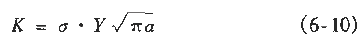
It can be seen from the formula (6-10) that the actual working stress can be known by knowing the shape of the member, the crack form, the crack length and the magnitude of the stress intensity factor.
The shape factor Y in (6-10), the crack length a can be obtained from the actual test of the component and the fracture. The key is how to use the fracture analysis to calculate the K value at any crack length.
According to the definition of fracture mechanics

among them
 For the cycle characteristics, if the R value can be determined, and K0 and Kmin can be calculated from (6-11) by calculating the ΔK from the microscopic picture analysis of the fracture using (6-9), obtain the formula (6-10). Actual working stress. The calculation procedure is shown in Figure 6-85.
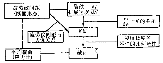
Figure 6-85 Procedure for estimating the load from the fatigue striation spacing
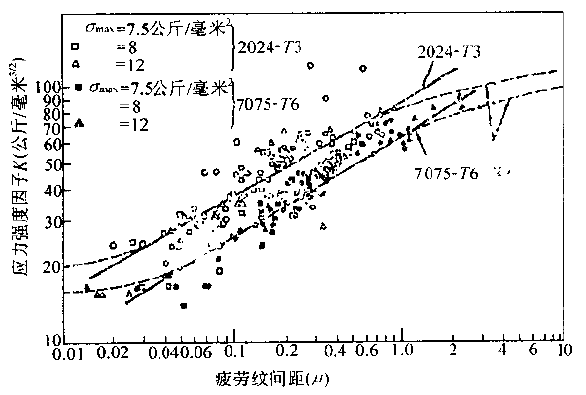
Figure 6-86 Relationship between fatigue fringe spacing and stress intensity factor
The experimental method is used to establish the relationship between the fatigue striation width and the K value. It has great reference value and application value for the quantitative load calculation of the actual fatigue fracture. Figure 6-86 is an actual test result. For comparison, the graph shows the crack macroscopic rate curve (dashed line), which is S-shaped. The upper end and the lower end of the curve deviate from the straight line, so in principle, quantitative analysis cannot be performed on the upper and lower ends. Fortunately, because their fracture morphology is significantly different from fatigue waviness, it is easy to distinguish them.
In a specific failure analysis, the R value can be determined by a specific analysis of the working mode of the component and the service conditions. In some special cases, it can be done. For example, according to the working characteristics of the gear, it can be inferred that the cyclic characteristic of the alternating load of the gear tooth root portion is R=σmin/σmax=0. The alternating load on the outer surface of the train axle and at any point inside is a symmetrical cycle of R=-1. For the case where the R value cannot be determined from the shape and working state of the component, further research work is required. In addition, many factors such as alternating frequency, overload event, ambient temperature and spectral load will affect the quantitative analysis of the fracture, which needs to be further explored.
Pool fences save lives. Experts recommend installing a pool safety fence as the best way to protect young children from drowning. Glass pool fences are a modern safety solution to prevent tragic accidents without blocking your view. Our Tempered Glass will be made to meet pool fence design, thickness, size, even with holes.
At present, 12mm TOUGHENED GLASS be chosen more for pool fence panels, hight about 1200mm, width different based on customer's request. And now, some customers also choose Laminated Glass , even SGP laminated glass for pool fence in some special areas, all can be made to request.
So Clear Tempered Glass , Colored Tinted Tempered Glass, Ultra Clear Tempered Glass, Clear Laminated Glass , Colored Laminated Glass , Low Iron Laminated Glass and so on, can also be choice based on request.
Reference photos:


Swimming Pool Fence Glass
Shanghai Lead Glass Co.,Ltd , https://www.leadglaze.com